First Order System Parameters Identification

Let's have some fun!

Hello everyone! This time we are going to estimate the parameters of a first order system from experimental data. For this experiment we use Scilab, Arduino and a RC circuit.

We start from the physical system as shown in the following figure 1. A $10 \space K\Omega$ resistor and a $100 \space \mu F$ capacitor are chosen.

Figure 1. RC Circuit.

The connections are shown in Figure 2.

Figure 2. RC Circuit Connections.

The circuit diagram is shown in Fig 3.

Figure 3. RC Circuit Diagram.

To obtain the differential equation of the circuit we use the resistor and capacitor $v-i$ relationships.

$Eq \space 1. \qquad V_R=iR$

$Eq \space 2. \qquad i=C \space \dot{V_C}$

Then, KVL

$Eq \space 3.  \qquad -V_S+V_R+V_C=0$

By subtituting $Eq \space 2$  in $Eq \space 1$ and the result in $Eq \space 3$, we obtain the differential equation of the system.

$Eq \space 4. \qquad RC \; \dot{V_C}+V_C=V_S$

Assuming zero initial conditions and applying the Laplace transform, we obtain the transfer function of the system.

$Eq \space 5. \qquad G(s) = \frac{V_C(s)}{V_S(s)}= \frac{1}{RC \space s+1}$

Analysis:

Figura 4. Open Loop System Block Diagram.

The step response of the open loop system is obtained as follows:

$Eq \space 6. \qquad V_C(s)=G(s) \cdot V_S(s)=\frac{1}{RC \space s+1} \cdot \frac{1}{s}$

If we substitute the values of $R=10 K\Omega$  and $C=100 \mu F$ in $Eq \space 6$ and then do the Partial-Fraction Expansion

$\hspace{42pt} V_C(s)=\frac{A}{s+1} + \frac{B}{s}$

$\hspace{42pt} A=\begin{equation} \left. {\frac{1}{s}}\right\rvert_{s=-1} \end{equation}= -1$

$\hspace{42pt} B=\begin{equation} \left. {\frac{1}{s+1}}\right\rvert_{s=0} \end{equation} = 1$

we get

$Eq \space 7. \qquad V_C(s)=\frac{-1}{s+1} + \frac{1}{s}$

applying the inverse Laplace transform to $Eq \space 7$

$Eq \space 8. \qquad \begin{equation} V_C(t)=1 -  e^{-t}\end{equation}$

The step response to the system of $Eq \space 8$ is shown in Figure 5.

Figure 5. RC Circuit Step Response (Eq 8).

Experiment:

Now, we use Scilab to acquire the data from the real system. The program is shown in Figure 6. We declare a sample time $Ts=0.02\,s$ for the data acquisition.

Figure 6. Scilab Xcos Data Acquisition Program.

The experiment consist of exciting the system with 5 volts from $t=0$ to $t=10$ seconds and the data is saved in the variable rcdata. The Experimental Input-Output Data is shown in Figure 7.

Figure 7. RC Circuit Experimental Input-Output Data.

As we can see, the first ten seconds of the Output in Fig 7 are similar to the Fig 5.

Identification:

To obtain the transfer function with the estimated parameters we need two things:
1. The steady state value.
2. The transient due to initial conditions.

Figure 8. Parameter Estimation.

The steady state value is used to identify the transfer function gain as follows.

$Eq \space 9. \qquad \begin{equation} K_{RC}= \frac{output
\,at\,steady\,state}{input\,at\,steady\,state}=\frac{4.9902}{5}=0.9980\end{equation}$

The free response due to initial condition is the data at $t>10$ seconds shown in Fig 8. This data is used to identify the system time constant $\tau$.

$Eq \space 10. \qquad  \begin{equation} \tau=RC= \frac{t_1-t_2}{\ln\left [\frac{c\,(t_2)}{c\,(t_1)} \right ] } = \frac{10.4396-10.9782}{\ln\left [\frac{2.2976}{3.7157} \right ] } = 1.12\,sec \end{equation}$

So, the system transfer function is

$Eq \space 11. \qquad  \begin{equation} G(s)=\frac{0.9980}{1.12\,s\,+\,1} \end{equation}$

Validation:

To validate the model, we excite the system of $Eq\,11$ with the same input of the experiment, and plot it against the output of the experiment. For this purpose we use the following Xcos program

Figure 9. Xcos Model Validation Program.

and the result is shown in the following figure

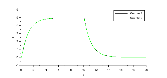Figure 10. Model Validation Plot.

As we can see in Figure 10, the model plot (green curve) is almost superposed to the experimental data (black curve). For this reason, the transfer function of $Eq\,11$ pretty much describes the system dynamics.

All the files used in this writing can be downloaded at the following link:
https://drive.google.com/open?id=1lg73aw6US3c5KHb82VSazmNkeMkHUnR1

Scilab Version: 5.5.2
Arduino toolbox by Bruno Jofret.